File paths and other constants to be used throughout the notebook
#!/usr/bin/env python
# -*- coding: utf-8 -*-

excelOriginal = '../data/imd_student_blind.xlsx'
csvOriginal = '../data/imd-student-blind.csv'
Libraries to import and use
# Import pandas
import pandas as pd
#Import numpy
import numpy as np
#import bokeh
from bokeh.plotting import figure
from bokeh.layouts import row
from bokeh.plotting import ColumnDataSource
from bokeh.models import HoverTool
from bokeh.models import Span, Label
from bokeh.charts import output_notebook, show, output_file, save
import warnings
from IPython.core.display import display, HTML

#disable annoying warnings
warnings.filterwarnings('ignore')

#alternative to output_notebook which loads html from file
def displayHTML(file):
    with open(file, 'r') as myfile:
        data=myfile.read()
        display(HTML(data))
2. Study directed to the subject '5'
So far, in this analysis, it has become clear that subject 5 is the most problematic for students, because it is in it that students have the worst performance. In this chapter, we will make an analysis directed to this subject.
2.1. Separation of students into two disjoint sets: Those who did well in subject 5 and those who did not do well
Start trying to statistically characterize the students who have performed well in it and those who have a poor performance. The function 'getGoodAndBadStudentsInDiscipline()' can use two criteria to determine whether a student has performed well or not:
- C1: Approved with a grade greater or equal to 7.0;
- C2: Approved on the first try;
df = pd.read_csv(csvOriginal)
def courseMedianGrade(df):
    return df['nota'].median()

def getDataframeForEachStudent(df, studentColumn='a_ID'):
    students = df.groupby(df['a_ID'])
    g = students.groups
    studentDFs = dict()
    for key, value in g.items():
        studentDFs[key] = students.get_group(key)
    return studentDFs

def eraseStudentsWhoDidNotParticipateOnClass(studentsDict, classID=5, classColumn='disciplina_ID'):
    before = len(studentsDict)
    toErase = list()
    for key, value in studentsDict.items():
        enrolled = False
        for label, row in value.iterrows():
            if((row[classColumn] == classID) or (row[classColumn] == str(classID))):
                enrolled = True
                #print("Student " + str(key) + " enrolled on " + str(classID))
                break
        if(not enrolled):
            toErase.append(key)
    for key in toErase:
        del studentsDict[key]
    print(str(before-len(studentsDict)) + " students did not enrolled on " + str(classID))
    return studentsDict

'''
standard   The criteria to determine if a student had a good performance or not
    'APPROVED ON FIRST TRY'
    'APPROVED WITH GRADE >= 7'
return     True if the student had a good performance
'''
def studentHadGoodPerformanceInDiscipline(studentDf, subject=5,
                                          standard='APPROVED WITH GRADE >= 7',
                                          classColumn='disciplina_ID'):
    if(standard == 'APPROVED ON FIRST TRY'):
        attempts = 0
        approved = False
        for label, row in studentDf.iterrows():
            if(row[classColumn] == subject):
                attempts = attempts + 1
                if(row['status.disciplina'] == 'Aprovado'):
                    approved = True
        return (approved and (attempts == 1))
    elif(standard == 'APPROVED WITH GRADE >= 7'):
        approved = False
        for label, row in studentDf.iterrows():
            if(row[classColumn] == subject):
                if(row['status.disciplina'] == 'Aprovado'):
                    if(row['nota'] >= 7.0):
                        approved = True
                        break
        return approved
    else:
        return False

'''
Given a class, separate the students between the ones who had a good performance on it, and the ones who did not.
'''
def getGoodAndBadStudentsInDiscipline(df, subject=5, standard='APPROVED ON FIRST TRY'):
    studentsRaw = getDataframeForEachStudent(df)
    students = eraseStudentsWhoDidNotParticipateOnClass(studentsRaw, classID=subject)
    goodStudents = list()
    badStudents = list()
    for key, studentDF in students.items():
        if(studentHadGoodPerformanceInDiscipline(studentDF, standard=standard, subject=subject)):
            goodStudents.append(key)
        else:
            badStudents.append(key)
    print(str(len(goodStudents)) + " good students in subject " + str(subject))
    x = len(students)
    print(str((len(goodStudents)/x)*100) + "% good students.")
    return (goodStudents, badStudents)

print('Using APPROVED ON FIRST TRY')
t = getGoodAndBadStudentsInDiscipline(df, subject=5, standard='APPROVED ON FIRST TRY')
print('\nUsing APPROVED WITH GRADE >= 7')
t2 = getGoodAndBadStudentsInDiscipline(df, subject=5, standard='APPROVED WITH GRADE >= 7')
To select only students approved with a grade greater or equal to 7.0 (C1) resulted in a very limited set of students, only 17.4%.
Our objective is to find characteristics in the two sets of students (those with good performance and those without), so a criterion wich selects only a small group of less than 1/4 of the total may not reveal relevant data.
Because of this and taking into account that the median grade for subject 5 is only 2.20, we will use the other criterion (C2), which selected the reasonable amount of 36% of the students, to separate the students.
C2 generating a set of only 36% of students suggests that subject 5 is a "bottleneck" in the course, causing only a small part of the students who arrive to it to pass through it and delaying the progress in the course to almost 2 in each 3 students.
2.2. Comparing grades in the course with grades in subject 5 and student status
Next, to better visualize this data, we will generate a graph to better visualize the relation between the students' grades with their grade in the subject 5 and, possibly, with the abandonment of the course.
def getStudentMeanGrade(df, studentID, studentColumn='a_ID', columnClasses='disciplina_ID', columnValue='nota'):
    studentDF = df[df[studentColumn] == studentID]
    return studentDF[columnValue].mean()

def getStudentMeanOnDiscipline(df, studentID, disciplineID,
                               studentColumn='a_ID', columnClasses='disciplina_ID',
                               columnValue='nota'):
    studentDF = df[df[studentColumn] == studentID]
    disciplineDF = studentDF[studentDF[columnClasses] == disciplineID]
    return disciplineDF[columnValue].mean()

def getStudentStatus(df, studentID, studentColumn='a_ID', statusColumn='status'):
    studentDF = df[df[studentColumn] == studentID]
    for label, row in studentDF.iterrows():
        return row[statusColumn]

goodStudentsMeanSeries = pd.Series(name='meanGrade')
otherStudentsMeanSeries = pd.Series(name='meanGrade')
goodStudentsDiscSeries = pd.Series(name='meanGradeIn5')
otherStudentsDiscSeries = pd.Series(name='meanGradeIn5')
goodStudentsStatusSeries = pd.Series(name='status')
otherStudentsStatusSeries = pd.Series(name='status')

for student in t[0]:
    goodStudentsMeanSeries[str(student)] = getStudentMeanGrade(df, student)
    goodStudentsDiscSeries[str(student)] = getStudentMeanOnDiscipline(df, student, 5)
    goodStudentsStatusSeries[str(student)] = getStudentStatus(df, student)
for student in t[1]:
    otherStudentsMeanSeries[str(student)] = getStudentMeanGrade(df, student)
    otherStudentsDiscSeries[str(student)] = getStudentMeanOnDiscipline(df, student, 5)
    otherStudentsStatusSeries[str(student)] = getStudentStatus(df, student)

print("Good students mean grade " + str(goodStudentsMeanSeries.mean()))
print("Other students mean grade " + str(otherStudentsMeanSeries.mean()))
print("Good students mean grade (in 5) " + str(goodStudentsDiscSeries.mean()))
print("Other students mean grade (in 5) " + str(otherStudentsDiscSeries.mean()))
Generate the plot:
def plotStudentSet(f, df, color):
    circleDataSource = ColumnDataSource(df[df['status'] == 'ATIVO'])
    xDf = df[df['status'] == 'TRANCADO'].append(df[df['status'] == 'CANCELADO'])
    xDataSource = ColumnDataSource(xDf)
    diamondDf = df[df['status'] == 'FORMADO'].append(
        df[df['status'] == 'FORMANDO']).append(df[df['status'] == 'CONCLUIDO'])
    diamondDataSource = ColumnDataSource(diamondDf)
    f.x('meanGrade', 'meanGradeIn5', alpha=1.0, source=xDataSource, line_width=3,
        size=16, legend='Abandonment', line_color=color)
    f.circle('meanGrade', 'meanGradeIn5', alpha=0.3, source=circleDataSource,
             fill_color=color, size=22, legend='Active in the course', line_color=None)
    f.diamond('meanGrade', 'meanGradeIn5', alpha=1.0, source=diamondDataSource,
              fill_color=color, size=21, legend='Graduated or Graduating', line_color='#FFFFFF')
    return f

goodStudentsDF = pd.concat([goodStudentsMeanSeries, goodStudentsDiscSeries,
                            goodStudentsStatusSeries],axis=1)
otherStudentsDF = pd.concat([otherStudentsMeanSeries, otherStudentsDiscSeries,
                             otherStudentsStatusSeries],axis=1)

f = figure(x_axis_label='Mean Grade in Subject 5', y_axis_label='Mean Grade',
           title="Overall Grade x Subject 5 Grade x Status. "
           +"RED = Good Student, BLUE = Other Students")

f = plotStudentSet(f, goodStudentsDF, '#FF0000')
f = plotStudentSet(f, otherStudentsDF, '#0000FF')

hline = Span(location=courseMedianGrade(df), dimension='height', line_color='green', line_width=3, line_dash='dashed')
f.add_layout(hline)
f.add_layout(Label(x=courseMedianGrade(df)-0.15, y=7.0, text='Course Median Grade', angle=3.14159/2))

hline2 = Span(location=courseMedianGrade(df[df['disciplina_ID'] == 5]), dimension='width',
              line_color='green', line_width=3, line_dash='dashed')
f.add_layout(hline2)
f.add_layout(Label(x=6.8, y=courseMedianGrade(df[df['disciplina_ID'] == 5])+0.1, text='Subject 5 Median'))

tips=[('Mean Grade','@meanGrade'),
     ('Grade in disc. 5','@meanGradeIn5'),
     ('Status','@status')]

f.add_tools(HoverTool(tooltips=tips))
f.legend.location = "top_left"

output_file("../result/gradesXsubject5gradesXstatus.html", title="Overall Grade x Subject 5 Grade x Status. "
           +"RED = Good Student, BLUE = Other Students")
save(f)
displayHTML('../result/gradesXsubject5gradesXstatus.html')
This data show that all of the students, even the ones with good performance on subject 5, tend to have grades smaller than their average in subject 5. The exceptions, with grades in subject 5 bigger than their average, are few.
Most of the good students in subject 5 also have grades above the course's median, but a relevant fraction of the students above the course's median were not successful in subject 5.
With just two exceptions, the students graduating or graduated are between the students who are good in subject 5. Also, we can observe a relation between being below the median of subject 5 with abandoning the course, because most 'X's are located between the students who are below the median for subject 5. That only reinforces the idea that subject 5 is a "bottleneck" on the curriculum of the course.
2.3. The 'Bottleneck Effect'
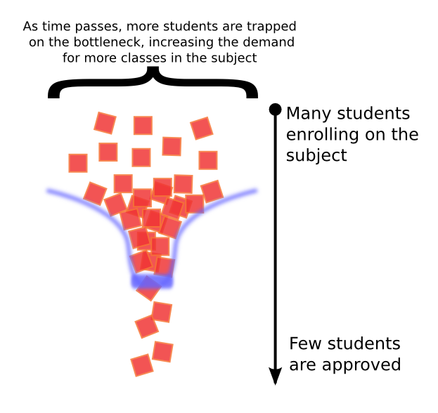
As the figure describes, each semester, a large amount of students needs to enroll on subject 5, but only a small part of them gets approved. The students who cannot get approved on their first try end up needing to enroll next semester, Occupying vacancies on the next semester with the new students. If the approval rate keeps being so low, the effect can acumulate successively, increasing the demand for new vacancies for subject 5.
2.4. Progression of students enrolled and approval rate for subject 5
def getStudentsEnrolledOnSemester(df, subject, year, period):
    subjectDF = df[df['disciplina_ID'] == subject]
    yearDF = subjectDF[subjectDF['ano_disciplina'] == year]
    periodDF = yearDF[yearDF['periodo_disciplina'] == period]
    total = 0
    for label, row in periodDF.iterrows():
        total = total + 1
    return total

nStudentsSeries = pd.Series(name="nStudents")
nStudentsSeries['2014.0'] = getStudentsEnrolledOnSemester(df, 5, 2014, 1)
nStudentsSeries['2014.5'] = getStudentsEnrolledOnSemester(df, 5, 2014, 2)
nStudentsSeries['2015.0'] = getStudentsEnrolledOnSemester(df, 5, 2015, 1)
nStudentsSeries['2015.5'] = getStudentsEnrolledOnSemester(df, 5, 2015, 2)
nStudentsSeries['2016.0'] = getStudentsEnrolledOnSemester(df, 5, 2016, 1)
nStudentsSeries['2016.5'] = getStudentsEnrolledOnSemester(df, 5, 2016, 2)
nStudentsSeries.index.name = 'Period'
nStudentsSeriesDF = pd.DataFrame(nStudentsSeries)
nStudentsSeriesDF.index = nStudentsSeriesDF.index.astype(float)

f = figure(x_axis_label='Period', y_axis_label='Students', title='Students on Subject 5',
           plot_width=400, plot_height=400)
f.line('Period', 'nStudents', source=ColumnDataSource(nStudentsSeriesDF), line_width=3)
f.circle('Period', 'nStudents', source=ColumnDataSource(nStudentsSeriesDF), fill_color="white", size=12)

print(nStudentsSeriesDF)
def getApprovalRateOnSemester(df, subject, year, period):
    subjectDF = df[df['disciplina_ID'] == subject]
    yearDF = subjectDF[subjectDF['ano_disciplina'] == year]
    periodDF = yearDF[yearDF['periodo_disciplina'] == period]
    total = 0
    approved = 0
    for label, row in periodDF.iterrows():
        if(row['status.disciplina'] == 'Aprovado'):
            approved = approved + 1
        total = total + 1
    if(total == 0 or approved == 0):
        return 0.0
    else:
        return approved/total

approvalSeries = pd.Series(name="approval-rate")
approvalSeries['2014.0'] = getApprovalRateOnSemester(df, 5, 2014, 1)*100
approvalSeries['2014.5'] = getApprovalRateOnSemester(df, 5, 2014, 2)*100
approvalSeries['2015.0'] = getApprovalRateOnSemester(df, 5, 2015, 1)*100
approvalSeries['2015.5'] = getApprovalRateOnSemester(df, 5, 2015, 2)*100
approvalSeries['2016.0'] = getApprovalRateOnSemester(df, 5, 2016, 1)*100
approvalSeries['2016.5'] = getApprovalRateOnSemester(df, 5, 2016, 2)*100
approvalSeries.index.name = 'Period'
approvalDF = pd.DataFrame(approvalSeries)
approvalDF.index = approvalDF.index.astype(float)
print(approvalDF)
f2 = figure(x_axis_label='Period', y_axis_label='Approval Rate (%)', title='Approval Rate on Subject 5',
           plot_width=400, plot_height=400)
f2.line('Period', 'approval-rate', source=ColumnDataSource(approvalDF), line_width=3)
f2.circle('Period', 'approval-rate', source=ColumnDataSource(approvalDF), fill_color="white", size=12)
output_notebook()
show(row(f,f2))
2.5. Some thoughts on the results found
The approval rate for subject 5 was worse back in 2016.1, 18%, and soon after it rised to 28%, in 2016.2. But its still observable that, in general, the rate has been decreasing. In 2014.1, the approval rate was of 48%.
As said early, the "bottleneck effect" can make the necessity for classes to subject 5 increase each semester. And with the decrease on the approval rate itself, the "bobbleneck effect" can get worse.
The increase in the necessity for vacancies for subject 5 can lead to a growing allocation of human (professors) and fisical (classrooms) resources from the course, which could be useful for other porpuses. This necessity for more resources, added to the high abandonment of the course in consequence of performance below the median, leads to the conclusion that the current situation of subject 5 is far from the ideal and prejudices the course of Bachelor in Information Technology as a whole.